Preparing the IO tables
Every country enters the model as a national IO table, but countries don’t all start from the same kind of table. The first step is to collect the best available table for each country and record where it came from: the source, version, year, valuation, and sector detail. Which table we start from depends on the country’s tier: the U.S. starts from Make and Use tables for 2024 that Cornerstone produces using BEA’s methodology, after redefinitions and following BEA’s 2017 detailed schema, while other countries start from national statistical agency tables, FIGARO or ICIO, or a template. See IO sources by country tier for what each tier starts from.
The detailed U.S. structure sets the model’s common sector list, and it is used to split other countries’ coarser sectors (see ABSR). Sector lists and currencies are reconciled in the later steps: mapping to the common sector list, linking with trade data, and balancing.
What’s in the tables
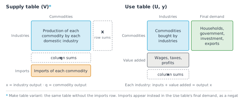
Figure 1:The Supply and Use tables. Supply shows who makes each commodity; Use shows who buys it and what each industry adds in value. The Make table (*) is a variant of Supply that leaves imports to the Use table.
An economy’s IO accounts come as a pair of tables.
Supply (V) records the production of each commodity by each domestic industry, plus imports of each commodity. The Make table, used for the U.S., is a variant: it has the same production block but no imports row. Imports appear instead in the Use table’s final demand, as a negative column. Either way, the production block gives two output totals:
Industry output
x: the sum across an industry’s row, which is everything the industry makes, including secondary products.Commodity output
q: the sum down a commodity’s column, which is everything domestic industries make of that commodity. Adding imports gives the total supply of the commodity.
Use (U and y) records who buys each commodity:
Intermediate use (
U): the commodities each industry buys as inputs.Final demand (
y): the commodities bought by final users, namely households, government, investment, and exports.Value added: below each industry’s inputs, its wages, taxes on production, and profits.
The two tables balance. For each commodity, total supply equals total use. For each industry, inputs plus value added equal the industry’s output x.
Domestic and imported use
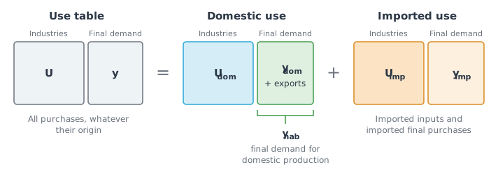
Figure 2:The Use table is split into domestic and imported use, for industries and final users alike.
A purchase can come from a domestic producer or from abroad, and the two lead to different supply chains. So the Use table is split in two:
Domestic use (
Udom,ydom): commodities bought from domestic producers.Imported use (
Uimp,yimp): commodities bought from producers in other countries.
U = Udom + Uimp. Final demand splits the same way, with exports on the domestic side: y = ydom + exports + yimp. Imported use is later traced back to the countries that made the imports, using trade data. How each country’s tables arrive at this split is described in IO sources by country tier.
From tables to direct requirements (A)
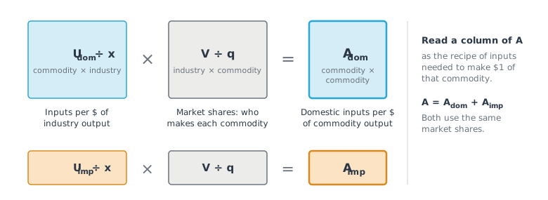
Figure 3:Domestic and imported direct requirements are built from the same two steps.
The direct requirements tables turn the Supply and Use tables into recipes: the inputs needed to make $1 of each commodity. They take three steps.
Inputs per dollar of industry output. Divide each industry’s column of domestic use by its output
x.Market shares. Divide each commodity’s column of the Supply table by its output
q. This gives the share of each commodity made by each industry.Combine. Multiply the two to get inputs per dollar of each commodity. Doing this with domestic use gives
Adom; doing it with imported use givesAimp.
For more details on the math behind it, contact team@cornerstonedata
Adom and Aimp add up to the total direct requirements A. A column of A is the input recipe for $1 of that commodity, split by where the inputs come from.
Tables that are already symmetric, with the same sectors on rows and columns, skip step 2: their domestic and imported use are divided by output directly. This applies to the Tier 1 and Tier 2 tables.
Final demand for the national accounting balance
Final demand in the Use table includes purchases of imports. To match domestic production, we need final demand for domestic products only. We call this ynab, the final demand for the national accounting balance: domestic final demand for domestic products (ydom) plus exports.
Here ydom is what households, government, and investment buy from domestic producers, and yimp is what they buy from abroad. Imports not bought by industries go to final users, so yimp is total imports less the row sums of Uimp. Exports are the country’s own production, so they count toward ynab in full.
With ynab, the model reproduces the country’s commodity output: running ynab through the domestic supply chain (the Leontief inverse of Adom) gives back q. This is a check that the tables, Adom, and ynab are consistent.
From single-country tables to the multi-region model
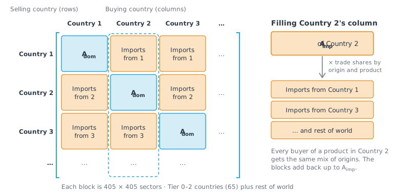
Figure 4:The MRIO direct requirements table. Each country’s domestic inputs sit on the diagonal; its imported inputs are spread down its column by country of origin.
Each country’s tables say how much of its inputs are imported, but not where they come from. The multi-region model links the countries so that a supply chain can be followed across borders.
Put every country in one table. The 65 countries in Tiers 0 to 2 each get their own block, so
Ais a 65 × 65 grid of country blocks, each 405 × 405 sectors. Each country’sAdomsits on the diagonal. A country’s column holds everything its industries buy; the rows say which country sold it.Split imports by origin. Each country’s
Aimpis spread down its column using bilateral trade data (BACI): for each product, the share the country imports from each origin. Products the trade data don’t cover, mostly services, use origin shares from FIGARO or ICIO. Imported final demand (yimp) is split the same way.Add the rest of the world. Imports from countries outside the table come from a rest-of-world region. Its domestic input structure is pooled from the tables of Colombia, Mexico, Türkiye, and Chile. It is added as one more block, making
Aa 66 × 66 grid of country blocks. This region is separate from the template used for Tier 3 countries’ own factors (see IO sources by country tier).Balance. The table is balanced with RAS, so that each country’s sales to all users, at home and abroad, add up to its output, without changing it’s domestic recipe. This makes small adjustments to the import coefficients.
Solve. The total requirements (
L) are calculated for the whole table at once, so supply chains that cross several borders are captured in full (see below).
The other 83 of the model’s 148 countries (Tier 3) are linked to this table more simply; see IO sources by country tier.
Total requirements (L)
A shows only a sector’s direct suppliers. Take $1 of furniture. Its column of A lists what the furniture maker buys to make it: lumber, hardware, electricity, transport. These are the first tier of the supply chain.
Each of those suppliers has its own column in A. The sawmill buys logs, fuel, and machinery; the power plant buys fuel and equipment. These purchases are the second tier. Each supplier’s column is scaled by how much of it the first tier needs: if the furniture maker buys 20 cents of lumber for each $1 of furniture, the sawmill’s whole recipe is multiplied by 0.20. The second-tier suppliers have their own suppliers, the third tier, scaled again by what the second tier needs, and so on, without end. In the multi-region model the trace crosses borders: a second-tier supplier may be a steel mill in another country.
Each tier is smaller than the one before, because every dollar of output pays for value added (wages, taxes, profits) as well as purchases. So the tiers add up to a finite total: everything produced, anywhere in the supply chain, to deliver $1 of each commodity to a final user. Written out, that total is I + A + A² + A³ + …, where I is the $1 of the commodity itself, A the first tier, A² the second, and so on.
There is a simple way to calculate this infinite sum all at once: a special inverse of A, (I − A)⁻¹, called the Leontief inverse after the economist Wassily Leontief. That is why the result is called L. A column of L shows the total output needed from every sector, in every country, for $1 of final demand for that commodity.
Key assumptions
Industry technology
Assumption: An industry uses the same input recipe for everything it makes, its primary product and any secondary products alike. This is what lets the market shares (
V÷q) turn industry recipes into commodity recipes.Why we make it: It is the standard assumption for building commodity-by-commodity tables from Supply and Use tables, and unlike the alternative (commodity technology) it never produces negative requirements.
How it affects results: A secondary product takes on its producer’s recipe. Using U.S. tables after redefinitions keeps secondary products, and so this effect, small.
Import proportionality
Assumption: Within a country, every buyer of a product gets the same mix of origins. If a country imports 30% of its steel from Korea, every industry that buys imported steel gets 30% of it from Korea.
Why we make it: Trade data record which countries trade each product, but not which industry buys the imports.
How it affects results: An industry that in reality buys mostly from one origin gets the national average mix instead. Where origins differ a lot in emission intensity, this can move that industry’s factors.
The rest of the world looks like four proxy economies
Assumption: The rest-of-world region stands in for every country outside the multi-region table, including all Tier 3 countries, as a source of imports. Its input recipe and emission intensities are pooled from Colombia, Mexico, Türkiye, and Chile. It buys nothing from other regions, so a supply chain that reaches it stays there.
Why we make it: Countries outside the table have no linked IO tables of their own, and these four are the lower-income OECD economies in the table.
How it affects results: Imports from Tier 3 countries carry the proxy economies’ emission intensities rather than their own. Supply chains can’t be traced to individual Tier 3 countries, or onward from the rest of the world to other regions.
Data-year recipes, shares, and intensities still apply in 2024
Assumption: The IO tables, emissions, trade shares, and gap-fill shares come from different years (for example, 2024 trade data with IO tables and emissions from 2018 to 2023). We assume the input recipes, origin shares, and emission intensities from each source’s data year still describe the 2024 economy. Each country’s emissions are divided by its output from the same year; that output is re-priced to 2024 dollars with a U.S. price index, so its direct emission intensities are data-year intensities per 2024 dollar.
Why we make it: National tables, multi-regional databases, and trade data are published on different schedules, and we use the most recent of each.
How it affects results: Where an economy’s structure, trading partners, or emission intensity changed between the data year and 2024 (for example, a cleaner electricity grid), the model reflects the earlier pattern. Using one U.S. price index for every country means price changes elsewhere are not captured. The years used for each country are listed in Methods by country.
Learn more
Supply, Use, and IO tables in national accounts - the United Nations Handbook United Nations, 2018
The standard textbook on IO analysis Miller & Blair, 2022;
How BEA builds the U.S. IO accounts BEA, 2009
- United Nations. (2018). Handbook on Supply, Use and Input-Output Tables with Extensions and Applications (No.74, Rev.1). Department of Economic and Social Affairs Statistics Division. https://unstats.un.org/unsd/nationalaccount/docs/SUT_IOT_HB_wc.pdf
- Miller, R., & Blair, P. (2022). Input-Output Analysis: Foundations and Extensions (3rd ed.). Cambridge University Press. https://www.cambridge.org/us/universitypress/subjects/economics/econometrics-statistics-and-mathematical-economics/input-output-analysis-foundations-and-extensions-3rd-edition?format=HB&isbn=9781108484763
- BEA. (2009). Concepts and Methods of the U.S. Input-Output Accounts. U.S. Bureau of Economic Analysis (BEA). https://www.bea.gov/resources/methodologies/concepts-methods-io-accounts